Logistic Regression

Written March 13, 2016

This post covers week 3 of Andrew Ng's excellent Coursera course on machine learning. You should read this post if the videos went too fast for you. To understand this post, you should know how linear regression works. If you don't, read this post first.

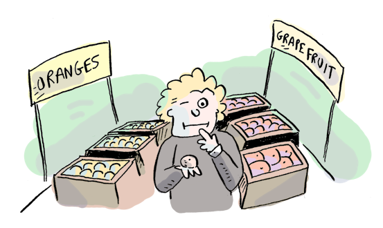
Logistic "regression" is classification algorithm. You can use it to classify things:

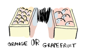
So instead of trying to predict a number (what price should I sell my house for?), you are trying to classify something (hey is this a grapefruit?).

Just to recap, linear regression is simple: you take your data, and plot it on a graph. Then you draw a line that fits your data pretty well. Now you can use that line to predict things. So you could use this line to predict housing prices based on size:

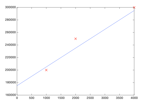
The best line is the one that minimizes a cost. For linear regression, the cost was the distance from each point of data to the line.

Similarly, when you are trying to classify something, first you plot your data on a graph.

Suppose you are trying to classify a new piece of fruit as an orange or a grapefruit. Here's your existing data:

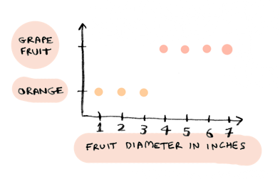
i.e. anything that is less than 4 inches in diameter is an orange, anything greater than that is a grapefruit.

Now you can draw a line in this image. Anything to the left of the line is an orange, and anything to the right is a grapefruit:

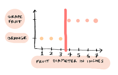
This is how logistic regression works. You plot your data, then draw a line. This line is called a decision boundary, and it splits the data into different classes (in this case, oranges and grapefruit).

Just like linear regression, logistic regression involves trying to find a line: except in this case, it is the decision boundary.

Prediction function

For the linear regression example, our data looked like this:

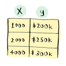
i.e. home size -> price of home.

For this example, our data looks like this:

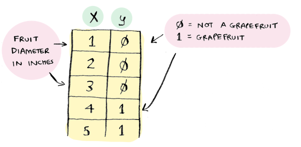
i.e. fruit diameter -> is it a grapefruit. If the fruit is a grapefruit, y = 1. Otherwise, y = 0.

In the linear regression example, we predicted a number (like a 3000 sq ft home will sell for $270,000). For logistic regression, we predict a probability, like "there's a 90% chance that this is a grapefruit".

In linear regression, the prediction formula looked like this:

You would calculate values for theta_0 and theta_1, and then use them to make a prediction. For example, if we wanted to know how much to sell a 3000 sq foot house for:

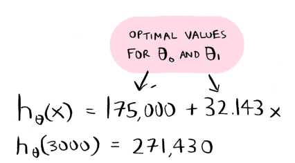
Once you had the optimal values for theta_0 and theta_1, the prediction part was easy.

We use almost the same formula for logistic regression, with one change:

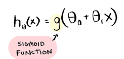
Remember, the prediction function for logistic regression spits out a percentage. As in "we are 95% sure this is a grapefruit". The g(...) is called the sigmoid function. This function is what makes the prediction function output a percentage. The sigmoid function constrains the result to between 0 and 1. So a result of .95 would mean we are 95% certain of something. That's all you really need to know about the sigmoid function.

The sigmoid function is:

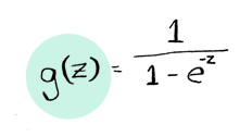
Just like linear regression, we will use a cost function to find good values for theta_0 and theta_1. But for our first example, I already know two good values. So lets plug them in:

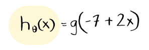
theta_0 = -7 and theta_1 = 2. Now we can use this function to predict whether a fruit is a grapefruit! Here are the results, for fruits of sizes 1 to 5 inches in diameter:

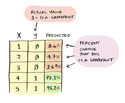
You can try this yourself by just plugging the numbers into WolframAlpha.

Remember, that percentage is your confidence that this fruit is a grapefruit. That's pretty close! The line looks like this:

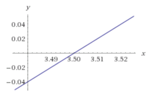
That's on the nose. Anything to the left of the line is an orange, and anything to the right is a grapefruit. Remember, the sigmoid function converts that into probabilities. The farther left you get, the more lower the percentage that the fruit is a grapefruit. So the sigmoid function smooths out the answers, instead of just spitting out a yes or a no:

So now that we have seen the prediction function in action, lets see how to find those optimal values for theta_0 and theta_1. Just to recap, the only thing we have changed so far is the prediction function h(x), to add the sigmoid function. Everything else is still the same as linear regression. The next thing we need to change is the cost function.

The cost function

In linear regression, we calculated the cost of using a line:

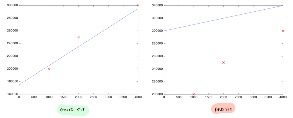
The cost was based on how far off the line was from our data points.

In logistic regression, the cost again depends on how far off our predictions are from our actual data. But we are using percentages, so the cost is calculated a little differently.

For example, if we say "There's a 95% chance that this is a grapefruit", but it turns out to be an orange, we should get penalized heavily (i.e. the cost should be higher). But if we say "There's a 55% chance that this is a grapefruit" and it turns to be an orange, that should be a lower penalty (i.e. the cost should be lower).

So the cost for logistic regression is calculated based on how far off your probability was. We calculate it using a log scale, like this:

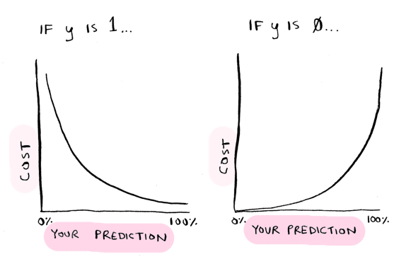
y is the actual result. So if y = 1 i.e. it was a grapefruit, and you predicted 1 (i.e. 100% probability it is a grapefruit), there's no penalty. But if you predicted 0 (0% probability it is a grapefruit), then you get penalized heavily.

The wronger you are, the more you get penalized. We use the log function for this.

The cost function for linear regression was:

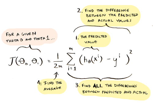
The cost function for logistic regression is:

And there's a clever way to write that on one line, like this:

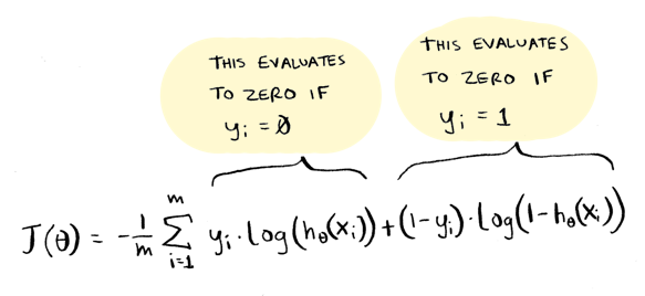
This works because one of those two will always be zero, so only the other one will get used, just like in the if statement. I personally prefer the if statement approach, but the videos use the one-liner so I've included it here.

Here it is in Octave:

function distance = cost(theta_0, theta_1, x, y)
  distance = 0;
  for i = 1:length(x) % arrays in octave are indexed starting at 1
    % you calculate the cost differently based on whether the actual value is 1 or 0.
    if (y(i) == 1)
      distance += -log(h(x(i), theta_0, theta_1));
    else
      distance += -log(1 - h(x(i), theta_0, theta_1));
    end
  end
  % get how far off we were on average
  distance = distance / length(x);
end

To recap:

We added the sigmoid function to the prediction function, so it outputs percentages
We changed the cost function (used the log function instead of predicted - actual)

That's it! Those two things are different, everything else is the same. We still use gradient descent to iteratively find the correct values for theta (and even the gradient descent formula still stays the same).

Here's the full example in Octave.

Now you know how to build a logistic regression classifier!

Multi-class classification

You know how logistic regression works now. The rest of this post is optional, and talks about some things you will run into when using logistic regression in practice.

How would you use logistic regression to classify between many different types of fruit, not just two different types?

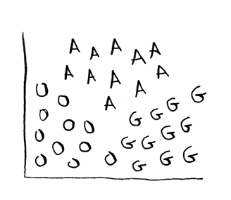
(O = orange, G = grapefruit, A = apple).

Then you need multiple decision boundaries:

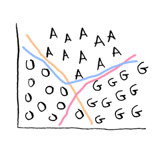
Turns out there's a really easy way to do this using something called one-vs-all classification! Here's the idea. First, just concentrate on grapefruit:

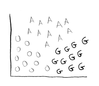
So either the fruit IS an grapefruit, or ISN'T an grapefruit (oranges and apples temporarily get lumped together). You do this classification and get a numbe, lets say 25%. So there's a 25% chance this is a grapefruit, and there's a 75% chance this is something other than a grapefruit.

Next you do the same with oranges:

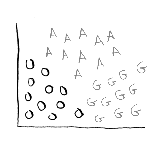
So either it IS an orange, or ISN'T (grapefruits and apples get lumped together). The output is 75%.

Finally, do this for apples:

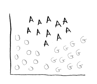
And you get: 30%.

So there's a 25% chance this is a grapefruit, 75% chance this is an orange, and 30% chance this is an apple. The result: it is an orange!

Non-linear classification

Suppose your data set looks like this:

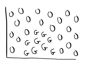
There's no straight line that you can use as your decision boundary. You need a non-linear boundary, like this:

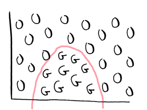
You can do this with logistic regression like this.

It uses a slightly different formula for prediction:

But in general it is really hard to do non-linear classification using logistic regression. Logistic regression is not good for something like this:

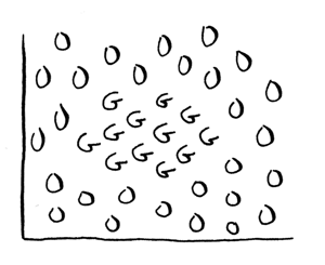
This is where non-linear classifiers shine. Neural networks and support vector machines (SVMs) are both good at non-linear classification.

Recap